The Pretty Good and Pretty Bad Measurements

In this tutorial, we will explore the “pretty good measurement” (PGM) and its novel counterpart, the “pretty bad measurement” (PBM). The PGM, also known as the square-root measurement, is a widely used measurement for quantum state discrimination [1][2]. The PBM, in contrast, was recently introduced by McIrvin et. al. [3]. Both these measurements provide elegant, easy-to-construct tools for two opposing goals in quantum information: state discrimination and state exclusion. PGM is useful for the former while PBM is of use for the latter.

We will verify their core properties and replicate some of the key numerical results and figures from the paper using |toqito⟩.

Background: Discrimination vs. Exclusion

Bob wins the standard quantum state discrimination task, if he successfully guesses the state sent by Alice. Alice is sending Bob a quantum state \(\rho_i\) chosen from an ensemble \(\{(p_i, \rho_i)\}_{i=1}^k\) known to Bob. Bob’s goal is to perform a measurement that maximizes his probability of correctly guessing the index \(i\). The best possible probability, \(P_{\text{Best}}\), is the maximum success probability achievable over all possible measurements (POVMs) \(\{M_i\}\).

\[P_{\text{Best}} = \max \sum_{i=1}^k p_i \text{Tr}(M_i \rho_i)\]

However, finding \(P_{\text{Best}}\) is often computationally very hard. The “pretty good measurement” (PGM) is a well-established heuristic for this task. Its measurement operators \(G_i\) are constructed from the ensemble as:

\[G_i = P^{-1/2} (p_i \rho_i) P^{-1/2} \quad \text{where} \quad P = \sum_{i=1}^k p_i \rho_i\]

The success probability when using the PGM is given by the standard Born rule, averaged over the ensemble:

\[P_{\text{PGM}} = \sum_{i=1}^k p_i \text{Tr}(\rho_i G_i)\]

The state exclusion task is the opposite: Bob wins if he correctly guesses a state that Alice did not send. This is equivalent to minimizing the probability of correctly guessing the state Alice did send. This minimum achievable success probability is denoted \(P_{\text{Worst}}\):

\[P_{\text{Worst}} = \min \sum_{i=1}^k p_i \text{Tr}(M_i \rho_i)\]

The “pretty bad measurement” (PBM) is a heuristic designed to approximate this worst-case performance. The PBM is elegantly defined in terms of the PGM operators \(G_i\). In the formula below, \(k\) is the number of states in the ensemble, and \(\mathbb{I}\) is the identity operator with the same dimensions as the states:

\[B_i = \frac{1}{k-1}(\mathbb{I} - G_i)\]

The success probability for discrimination when using the PBM is, analogously:

\[P_{\text{PBM}} = \sum_{i=1}^k p_i \text{Tr}(\rho_i B_i)\]

A key result from McIrvin et.al [3] is the tight relationship between the success probabilities of these two measurements:

\[P_{\text{PGM}} + (k-1)P_{\text{PBM}} = 1\]

This implies a performance hierarchy against the optimal probabilities and the blind guessing probability (\(1/k\)):

\[P_{\text{Best}} \ge P_{\text{PGM}} \ge \frac{1}{k} \ge P_{\text{PBM}} \ge P_{\text{Worst}}\]

We will verify this hierarchy with a concrete example.

Numerical Example: The Trine States

Figure 3 from McIrvin et.al [3] analyzes the performance of these measurements for the three trine states with a uniform prior probability. The trine states are a classic example of a set that is antidistinguishable but not distinguishable, a property demonstrated in the Quantum state exclusion tutorial.

Our plan is to:

1. Generate the trine states and assume uniform prior probabilities.

2. Compute the optimal win/loss probabilities, \(P_{\text{Best}}\) and \(P_{\text{Worst}}\), using |toqito⟩’s SDP solvers.

3. Construct the PGM and PBM measurement operators.

4. Calculate the success probabilities \(P_{\text{PGM}}\) and \(P_{\text{PBM}}\).

5. Print and compare all values, verifying the performance hierarchy and the relationship between \(P_{\text{PGM}}\) and \(P_{\text{PBM}}\).

import numpy as np
from toqito.measurements import pretty_bad_measurement, pretty_good_measurement
from toqito.states import trine
from toqito.state_opt import state_distinguishability, state_exclusion


def calculate_success_prob(
    states: list[np.ndarray],
    probs: list[float],
    povm_operators: list[np.ndarray],
) -> float:
    """Calculate the success probability Σ pᵢ Tr(ρᵢ Mᵢ).

    This helper is robust to `states` being either state vectors or density matrices.
    """
    success_prob = 0
    num_states = len(states)
    for i in range(num_states):
        state = states[i]
        op = povm_operators[i]
        # Check if input is a vector (pure state) or matrix (density matrix)
        if state.ndim == 1 or (state.ndim == 2 and min(state.shape) == 1):
            # It's a vector (or column/row vector)
            state_vec = state.flatten()
            prob_i = state_vec.conj().T @ op @ state_vec
        else:
            # It's a density matrix
            prob_i = np.trace(op @ state)
        success_prob += probs[i] * prob_i
    return np.real(success_prob)


# 1. Define the states and probabilities.
state_vectors = trine()
k = len(state_vectors)
probs = [1 / k] * k

print(f"Analyzing k={k} trine states with uniform probability.")

# 2. Compute the optimal benchmark values.
p_best, _ = state_distinguishability(state_vectors, probs)
p_worst, _ = state_exclusion(state_vectors, probs)

print(f"\nOptimal Benchmarks:")
print(f"  P_Best  = {p_best:.4f} (Max discrimination probability)")
print(f"  P_Worst = {p_worst:.4f} (Min discrimination probability)")

Analyzing k=3 trine states with uniform probability.

Optimal Benchmarks:
  P_Best  = 0.6667 (Max discrimination probability)
  P_Worst = -0.0000 (Min discrimination probability)

The results for the optimal benchmarks show that the maximum possible success probability is \(2/3\), and the minimum is \(0\). The PGM is known to be optimal for the trine states, so we expect \(P_{\text{PGM}} = P_{\text{Best}}\).

# 3. Compute the PGM and PBM operators.
pgm_operators = pretty_good_measurement(state_vectors, probs)
pbm_operators = pretty_bad_measurement(state_vectors, probs)

# 4. Calculate PGM and PBM success probabilities.
p_pgm = calculate_success_prob(state_vectors, probs, pgm_operators)
p_pbm = calculate_success_prob(state_vectors, probs, pbm_operators)

print(f"\nHeuristic Measurements:")
print(f"  P_PGM = {p_pgm:.4f}")
print(f"  P_PBM = {p_pbm:.4f}")

Heuristic Measurements:
  P_PGM = 0.6667
  P_PBM = 0.1667

As expected, the PGM achieves the optimal value. Our calculated value for the PBM is \(1/6 \approx 0.1667\), which is a good approximation of the true worst case of \(0\).

Finally, we can verify the core relationship between these two measurements and the full performance hierarchy stated previously.

\[P_{\text{Best}} \ge P_{\text{PGM}} \ge \frac{1}{k} \ge P_{\text{PBM}} \ge P_{\text{Worst}}\]

# 5. Verify the core relationship and the hierarchy.
relation_lhs = p_pgm + (k - 1) * p_pbm
print(f"\nVerifying P_PGM + (k-1)*P_PBM = 1:")
print(f"  {p_pgm:.4f} + ({k - 1})*{p_pbm:.4f} = {relation_lhs:.4f} -> {np.isclose(relation_lhs, 1)}")

print("\nVerifying hierarchy (P_Best >= P_PGM >= 1/k >= P_PBM >= P_Worst):")
print(f"  P_Best >= P_PGM:    {p_best:.4f} >= {p_pgm:.4f}  ->  {p_best >= p_pgm or np.isclose(p_best, p_pgm)}")
print(f"  P_PGM >= 1/k:       {p_pgm:.4f} >= {1 / k:.4f}  ->  {p_pgm >= 1 / k or np.isclose(p_pgm, 1 / k)}")
print(f"  1/k >= P_PBM:       {1 / k:.4f} >= {p_pbm:.4f}  ->  {1 / k >= p_pbm or np.isclose(1 / k, p_pbm)}")
print(f"  P_PBM >= P_Worst:   {p_pbm:.4f} >= {p_worst:.4f} ->  {p_pbm >= p_worst or np.isclose(p_pbm, p_worst)}")

Verifying P_PGM + (k-1)*P_PBM = 1:
  0.6667 + (2)*0.1667 = 1.0000 -> True

Verifying hierarchy (P_Best >= P_PGM >= 1/k >= P_PBM >= P_Worst):
  P_Best >= P_PGM:    0.6667 >= 0.6667  ->  True
  P_PGM >= 1/k:       0.6667 >= 0.3333  ->  True
  1/k >= P_PBM:       0.3333 >= 0.1667  ->  True
  P_PBM >= P_Worst:   0.1667 >= -0.0000 ->  True

The verifications confirm that all theoretical relationships hold true for the trine states.

Now we can move on to visualizing the performance for the more general case of random states.

Visualizing Performance on Random States

Figures 4 and 5 from McIrvin et. al [3] show that for many randomly generated states, the PGM and PBM probabilities cluster around the blind guessing baseline of \(1/k\). We can reproduce a similar plot.

We will generate 100 random ensembles of \(k=4\) qubit states and plot the resulting \(P_{\text{PGM}}\) and \(P_{\text{PBM}}\) values.

import matplotlib.pyplot as plt

from toqito.rand import random_density_matrix

# Number of random ensembles to generate.
num_instances = 100
k = 4  # Number of states in each ensemble.
dim = 2  # Dimension of states (qubits).

pgm_results = []
pbm_results = []

for i in range(num_instances):
    # Generate a random ensemble of k density matrices.
    rand_states = [random_density_matrix(dim, seed=(i * k) + j) for j in range(k)]
    # Generate random prior probabilities.
    rand_probs = np.random.dirichlet(np.ones(k))

    # Calculate PGM and PBM probabilities.
    pgm_ops = pretty_good_measurement(rand_states, rand_probs)
    pbm_ops = pretty_bad_measurement(rand_states, rand_probs)

    pgm_prob = calculate_success_prob(rand_states, rand_probs, pgm_ops)
    pbm_prob = calculate_success_prob(rand_states, rand_probs, pbm_ops)
    pgm_results.append(pgm_prob)
    pbm_results.append(pbm_prob)

# Create the plot.
fig, ax = plt.subplots(figsize=(8, 5), dpi=100)
sample_indices = range(num_instances)
ax.scatter(sample_indices, pgm_results, alpha=0.7, label="$P_{PGM}$", c="blue", s=20)
ax.scatter(sample_indices, pbm_results, alpha=0.7, label="$P_{PBM}$", c="red", s=20)

# Add blind guessing line for reference.
blind_guess_prob = 1 / k
ax.axhline(
    y=blind_guess_prob,
    color="black",
    linestyle="--",
    label=f"Blind Guessing (1/k = {blind_guess_prob:.2f})",
)

ax.set_xlabel("Random Instance Index", fontsize=12)
ax.set_ylabel("Discrimination Success Probability", fontsize=12)
ax.set_title(f"PGM and PBM Performance for {num_instances} Random Ensembles (k={k})", fontsize=14)
ax.legend()
ax.grid(True, linestyle=":", alpha=0.6)
plt.tight_layout()
plt.show()

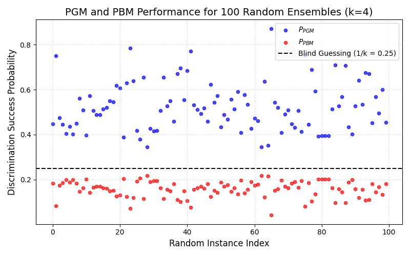
This plot clearly illustrates the theoretical bounds. Every blue dot representing \(P_{\text{PGM}}\) lies on or above the blind guessing line, and every red dot representing \(P_{\text{PBM}}\) lies on or below it. This provides strong numerical evidence for the inequalities \(P_{\text{PGM}} \ge 1/k \ge P_{\text{PBM}}\), confirming that the PGM is always a better-than-random guess and the PBM is always a worse-than-random guess for state discrimination.

References

[1]

V. P. Belavkin. Optimal distinction of non-orthogonal quantum signals. Radio Engineering and Electronic Physics, 20:39–47, 1975.

[2]

Lane P Hughston, Richard Jozsa, and William K Wootters. A complete classification of quantum ensembles having a given density matrix. Physics Letters A, 183(1):14–18, 1993.

[3] (1,2,3,4)

Caleb McIrvin, Ankith Mohan, and Jamie Sikora. The pretty bad measurement. 2024. arXiv:2403.17252.