The Pusey-Barrett-Rudolph (PBR) Theorem

In this tutorial, we will explore the Pusey-Barrett-Rudolph (PBR) theorem [1], a significant no-go theorem in the foundations of quantum mechanics. We will describe the theorem’s core argument and then use |toqito⟩ to verify the central mathematical property that the theorem relies on.

The PBR theorem addresses a fundamental question: Is the quantum state (e.g., the wavefunction \(|\psi\rangle\)) a real, objective property of a single system (an ontic state), or does it merely represent our incomplete knowledge or information about some deeper underlying reality (an epistemic state)?

PBR Argument

The PBR theorem [1] argues against a broad class of epistemic models.

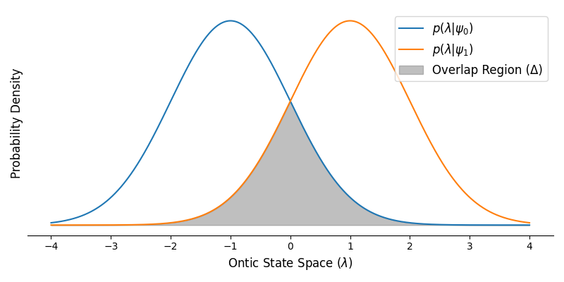
1. Epistemic Hypothesis: An epistemic model assumes there is a “real” physical state of the system, often denoted by \(\lambda\). The quantum state \(|\psi\rangle\) is then just a probability distribution over the possible values of \(\lambda\). A key implication is that the distributions for two different quantum states, say \(|\psi_0\rangle\) and \(|\psi_1\rangle\), could overlap. This means that for some underlying physical states \(\lambda\), the system could have been prepared in either \(|\psi_0\rangle\) or \(|\psi_1\rangle\).

   We can visualize the overlap of these hypothetical probability distributions. To do this, we will create a simple illustrative plot. We are not assuming any specific physical model for \(\lambda\); the plot is purely a visual aid to make the concept of overlapping probability distributions concrete.

   For this illustration, we represent the space of possible ontic states \(\lambda\) on the x-axis. We then choose two simple, overlapping normal (Gaussian) distributions to represent the hypothetical probability densities \(p(\lambda | \psi_0)\) and \(p(\lambda | \psi_1)\). The specific choice of Gaussian distributions is arbitrary; any pair of distinct, overlapping distributions would demonstrate the same essential feature.

import matplotlib.pyplot as plt
import numpy as np
from scipy.stats import norm

fig, ax = plt.subplots(figsize=(8, 4), dpi=100)
lambda_space = np.linspace(-4, 4, 1000)
dist_0 = norm(loc=-1, scale=1)
dist_1 = norm(loc=1, scale=1)
p_lambda_0 = dist_0.pdf(lambda_space)
p_lambda_1 = dist_1.pdf(lambda_space)
ax.plot(lambda_space, p_lambda_0, label=r"$p(\lambda | \psi_0)$")
ax.plot(lambda_space, p_lambda_1, label=r"$p(\lambda | \psi_1)$")
ax.fill_between(
    lambda_space,
    np.minimum(p_lambda_0, p_lambda_1),
    color="gray",
    alpha=0.5,
    label="Overlap Region (Δ)",
)
ax.set_xlabel(r"Ontic State Space ($\lambda$)", fontsize=12)
ax.set_ylabel(r"Probability Density", fontsize=12)
ax.set_yticks([])
ax.legend(fontsize=12)
ax.spines["top"].set_visible(False)
ax.spines["right"].set_visible(False)
ax.spines["left"].set_visible(False)
plt.tight_layout()

Note

The shaded region \(\Delta\) represents the set of ontic states \(\lambda\) that are ambiguous—the system could have been prepared as \(|\psi_0\rangle\) or \(|\psi_1\rangle\). The PBR theorem shows that the existence of any such overlap (for any pair of distinct states) leads to a contradiction with quantum theory’s predictions. Figure adapted from the PBR paper [1].

2. Thought Experiment: The PBR paper [1] constructs a thought experiment to show this leads to a contradiction. Consider two non-orthogonal quantum states, for example:

   \[|0\rangle \quad \text{and } \quad |+\rangle = \frac{1}{\sqrt{2}}(|0\rangle + |1\rangle)\]

   If their underlying reality distributions overlap, it’s possible to prepare a system where its true state \(\lambda\) is consistent with both preparations. Now, imagine we prepare two such systems independently. There is a non-zero chance that the combined physical state \((\lambda_1, \lambda_2)\) is compatible with any of the four possible quantum preparations:

   \[|0\rangle \otimes |0\rangle, \quad |0\rangle \otimes |+\rangle, \text{ } |+\rangle \otimes |0\rangle, \quad |+\rangle \otimes |+\rangle\]

3. Contradiction via Antidistinguishability: The crux of the theorem is to show that quantum mechanics allows for a special entangled measurement on the two systems. This measurement has a remarkable property: each of its possible outcomes is strictly forbidden (has zero probability) for at least one of the four product states.

   This property is known as antidistinguishability. A set of states \(\{|\Psi_i\rangle\}\) is antidistinguishable if there exists a measurement with outcomes \(\{M_i\}\) such that \(\langle \Psi_i | M_i | \Psi_i \rangle = 0\) for all \(i\).

   This leads to a contradiction:

   • The epistemic model predicts that sometimes the underlying reality \((\lambda_1, \lambda_2)\) is ambiguous.

   • In these cases, the measurement (which only depends on \(\lambda\)) must produce some outcome, say outcome \(k\).

   • But what if the state was actually prepared as \(|\Psi_k\rangle\)? Quantum mechanics says outcome \(k\) is impossible for this state.

   This contradiction implies that the initial assumption—that the distributions for \(|0\rangle\) and \(|+\rangle\) overlap—must be false. The PBR theorem generalizes this to any pair of distinct quantum states. The conclusion is that, under the assumption of preparation independence, the quantum state must be ontic.

Verifying Antidistinguishability with |toqito⟩

We can now use |toqito⟩ to verify the key requirement for the PBR theorem that the set of four states constructed from \(|0\rangle\) and \(|+\rangle\) are indeed antidistinguishable.

import numpy as np

from toqito.matrices import standard_basis
from toqito.matrix_ops import tensor
from toqito.state_props import is_antidistinguishable

# Define the single-qubit states |0> and |+>.
e_0, e_1 = standard_basis(2)
state_0 = e_0
state_plus = (e_0 + e_1) / np.sqrt(2)

# Construct the four 2-qubit product states from the PBR paper's simple example.
psi_00 = tensor(state_0, state_0)
psi_0_plus = tensor(state_0, state_plus)
psi_plus_0 = tensor(state_plus, state_0)
psi_plus_plus = tensor(state_plus, state_plus)

pbr_states = [psi_00, psi_0_plus, psi_plus_0, psi_plus_plus]

# Check if this set of states is antidistinguishable.
is_ad = is_antidistinguishable(pbr_states)

print(f"Are the four PBR states antidistinguishable? {is_ad}")

Are the four PBR states antidistinguishable? True

The result confirms that there exists a measurement that can perfectly exclude each of the four states, providing the necessary ingredient for the PBR no-go theorem’s contradiction.

This result, derived from a solvable semidefinite program within |toqito⟩’s state_exclusion() function supports the theorem’s conclusion that the quantum state has a strong claim to being an objective feature of reality.

General PBR States

The theorem holds for any pair of non-orthogonal states. The toqito library provides a function to generate the states from the more general proof in the PBR paper [1], which are defined by an angle \(\theta\).

\[|\psi_0\rangle = \cos(\frac{\theta}{2})|0\rangle + \sin(\frac{\theta}{2})|1\rangle \quad \text{and } |\psi_1\rangle = \cos(\frac{\theta}{2})|0\rangle - \sin(\frac{\theta}{2})|1\rangle\]

For instance, we can generate a set of \(2^n\) states for some \(n\) and \(\theta\).

from toqito.states import pusey_barrett_rudolph

# Generate states for n=2 systems and theta = pi/3
general_pbr_states = pusey_barrett_rudolph(n=2, theta=np.pi / 3)

The inner product of the two base states is \(\cos(\theta)\). For these to be antidistinguishable, we need to check the condition from the paper. The theorem states that if \(2^{1/n} - 1 < \tan(\theta/2)\), a contradiction is obtained. For \(n=2\) and \(\theta=\pi/3\), we have \(\tan(\theta/2) = \tan(\pi/6) \approx 0.577\). The other side of the inequality is \(2^{1/2} - 1 \approx 0.414\). Since \(0.414 < 0.577\), the theorem applies and this set should be antidistinguishable.

is_ad_general = is_antidistinguishable(general_pbr_states)

print(f"\nAre the four general PBR states (n=2, theta=pi/3) antidistinguishable? {is_ad_general}")

Are the four general PBR states (n=2, theta=pi/3) antidistinguishable? True

References

[1] (1,2,3,4,5)

Matthew F. Pusey, Jonathan Barrett, and Terry Rudolph. On the reality of the quantum state. Nature Physics, 8(6):475–478, May 2012. URL: http://dx.doi.org/10.1038/nphys2309, doi:10.1038/nphys2309.